Dealing with Noisy Data

Big data is almost always noisy. The techniques that work on small data should be adapted to overcome this noise. As an illustration, the simplest program we can think of to visualize the New York Taxi dataset is the follwing:

from progressivis import CSVLoader, Histogram2D, Min, Max, Heatmap

LARGE_TAXI_FILE = "https://www.aviz.fr/nyc-taxi/yellow_tripdata_2015-01.csv.bz2"
RESOLUTION=512


csv = CSVLoader(LARGE_TAXI_FILE,
                index_col=False,
                usecols=['pickup_longitude', 'pickup_latitude'])

min = Min()
min.input.table = csv.output.result

max = Max()
max.input.table = csv.output.result

histogram2d = Histogram2D('pickup_longitude', 'pickup_latitude',
                          xbins=RESOLUTION, ybins=RESOLUTION)
histogram2d.input.table = csv.output.result
histogram2d.input.min = min.output.result
histogram2d.input.max = max.output.result

heatmap = Heatmap()
heatmap.input.array = histogram2d.output.result

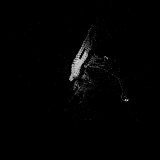
Instead of using the Quantiles module presented in the first example, it simply uses Min and Max to obtain the bounds of the pickup positions before computing the heatmap image. It works as well, but the resulting image is unexpected:

This is due to taxis driving to Florida (bottom right, sometimes invisible on high-resolution displays) or other far away places and forgetting to stop their meters. The Quantiles module allows getting rid of outliers that always exist in real data, that is always noisy.

Alternatively, you may know the boundaries of NYC and specify them:

from progressivis import CSVLoader, Histogram2D, ConstDict, Heatmap, PDict
from dataclasses import dataclass


LARGE_TAXI_FILE = "https://www.aviz.fr/nyc-taxi/yellow_tripdata_2015-01.csv.bz2"
RESOLUTION=512

@dataclass
class Bounds:
    top: float = 40.92
    bottom: float = 40.49
    left: float = -74.27
    right: float = -73.68

bounds = Bounds()
col_x = "pickup_longitude"
col_y = "pickup_latitude"


csv = CSVLoader(LARGE_TAXI_FILE,
                index_col=False,
                usecols=[col_x, col_y])

min = ConstDict(PDict({col_x: bounds.left, col_y: bounds.bottom}))
max = ConstDict(PDict({col_x: bounds.right, col_y: bounds.top}))

histogram2d = Histogram2D(col_x, col_y,
                          xbins=RESOLUTION, ybins=RESOLUTION)
histogram2d.input.table = csv.output.result
histogram2d.input.min = min.output.result
histogram2d.input.max = max.output.result

heatmap = Heatmap()
heatmap.input.array = histogram2d.output.result
...

The result is then perfect, but you need to provide extra information, i.e., the boundaries of the image.