Progressive Notebooks#
The best environment to use ProgressiVis is the Jupyter lab notebook with extensions supported in the package called ipyprogressivis.
The recommended way to get these extensions is to install ProgressiVis with the Jupyter option, as explained here.
This package provides ProgressiVis specific support for the user interface and visualizations, as well as components to explore CSV and Apache Arrow datasets.
Running Jupyter#
To meet the display requirements of progressive notebooks, it is essential to use Jupyter Lab (and not Jupyter Notebook).
Note
The cells in a ProgressiBook are created programmatically, which means that the ProgressiBook is not automatically trusted by Jupyter. Therefore, to obtain a satisfactory rendering of a previously created ProgressiBook, the file must be “trusted” by Jupyter. This can be done using the command line interface as follows:
jupyter trust /path/to/YourProgressiBook.ipynb
Alternatively, you can “trust” your file in the Jupyterlab interface via the menu View/Activate command palette/Search trust.
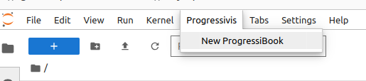
Creating a progressive analysis#
Notebooks hosting a progressive scenario need to be initialized in a particular way. We call them ProgressiBooks and they must be created via the Progressivis/New ProgressiBook menu, made available with ipyprogressivis:
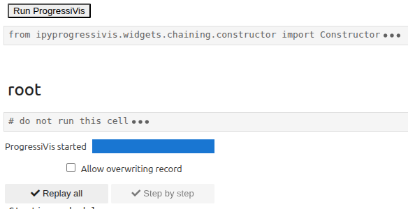
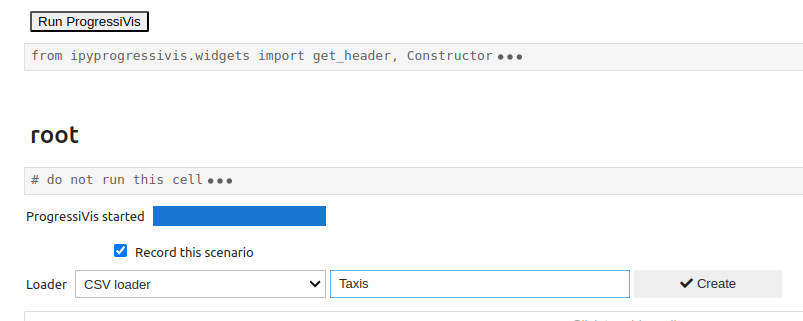
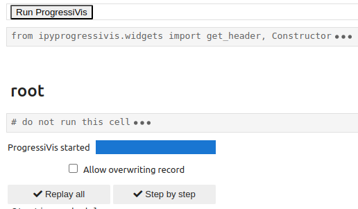
Once created, a Run ProgressiVis button will appear in the first ProgressiBook cell.
By clicking this button, ProgressiVis is launched, and the starting box will appear. A new scenario always begins by defining a data source. Currently, it proposes three data loading options. Two of them are predefined (CSV loader and PARQUET loader), and the third is the possibility to define (i.e., to code in Python) a customized loader. The starting box also offers the option of saving the session for later use by checking the record this scenario box. These actions, like all other actions in the scenario, are implemented via a set of chaining widgets.

Replaying a progressive analysis#
To replay a previously recorded scenario, you need to open the ProgressiBook like an ordinary notebook, which will contain a snapshot of the previous execution.
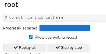
By pressing the Run ProgressiVis button, the snapshot will disappear, and the following box will appear instead :
Pressing the Replay all button will launch the recorded scenario, but you won’t be able to change it.
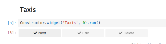
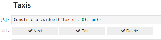
On the other hand, if you check the Allow overwriting record box, the Step by step button will become active:
You can choose between two modes:
Replay all: the recorded scenario will be launched as before, but you’ll be able to enrich it with new widgets.Step by step: the various nodes will be displayed in the order in which they were created in the initial scenario, and you can:run it identically by pressing
Nextmodify it (at your own risk) by choosing
Editdelete it (and its descendants) by choosing
Delete
Note
If you’ve chosen Step by step mode, you must run through all the nodes (except for deletions), otherwise you’ll end up with an incoherent scenario.
Do not cut and paste from a ProgressiBook to a standard Notebook#
ProgressiBooks are managed in a different way than normal notebooks. Copying a cell from a ProgressiBooks to a normal notebook will not work in general, not even to another ProgressiBook.
You can use ipyprogressivis widgets inside regular notebooks by importing the ipyprogressivis.view package.
TODO
Chaining widgets#
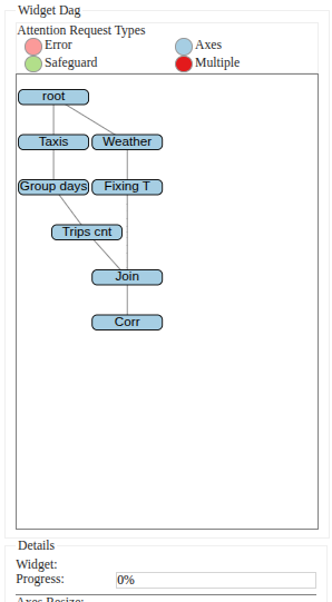
As their name suggests, chaining widgets (CW) are graphical components based on Jupyter widgets that can be composed to implement progressive data analysis scenarios. Their interconnection capabilities enable the creation of directed acyclic graphs (DAGs).
Each CW is designed for a specific stage of an analysis scenario (data loading, filtering, joins, etc.) and is associated with a sub-graph of ProgressiVis modules in the background, usually grouped behind a front panel.
Chaining widgets encapsulate and connect a subgraph of ProgressiVis modules that would take several line of code to create for no benefit.
A ProgressiBook user guide#
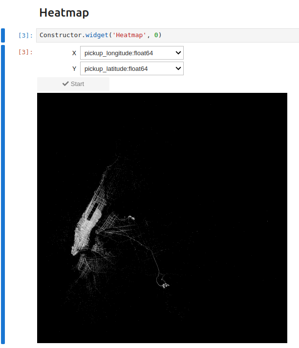
Let’s return to the scenario developed in the user guide, starting with the basic variant.
By combining two CWs: CSVLoader and Heatmap, we’ll reproduce the same behaviour (i.e., which doesn’t deal with the bounds issue).
Note
The CSVLoader features advanced configuration mechanisms (column selection, retyping, filtering, etc.) via the CSV sniffer, which is described in more details here
The notebook below is available and ready to run in the ipyprogressivis repository in notebooks/userguide-widgets1.0.ipynb:
To go further and take into account the (assumed known) bounds like the second snippet in the user guide, we can use the filtering capabilities available to the CSV sniffer this way:

Then renew the operation for pickup_latitude, click the Start loading csv button, chain with a Heatmap widget, configure it with the appropriate columns, and you get the expected result:
But if you don’t know the bounds a priori, you can eliminate the noise using quantiles like this python code does because a Quantile chaining widget is available. The notebook below shows this approach. It is available and ready to be replayed in notebooks/userguide-widgets1.1.ipynb
:
Finally, if you want to control the bounds dynamically, you can simply implement the third approach in the guide (see the Python code here) by assembling predefined widgets.
In concrete terms, instead of connecting Heatmap to the CSVLoader output, you need to insert a RangeQuery2D widget between the two widgets already mentioned, this way:

Chaining widgets list#
We give a summary of the chaining widgets available here.
Data loaders category#
There are three main loaders: the CSV loader, the PARQUET/Arrow loader, and custom loaders. For CSV and Arrow files, we provide additional functionalities to investigate the structure of the files and specify what columns to load, the concrete types to use, and more details.
CSV loader#
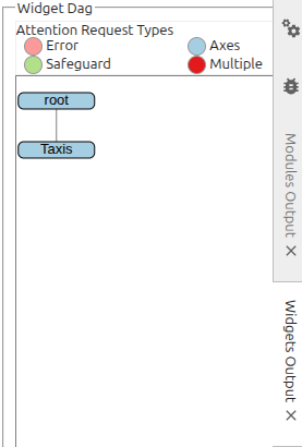
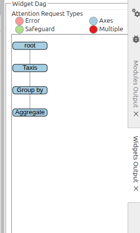
Usually, the first cell of a progressive analysis is a data loader, below the root, creating this possible topology:
Function:#
The CSV loader, as its name implies, loads one or many CSV files progressively.
After starting, the main interface looks like this:
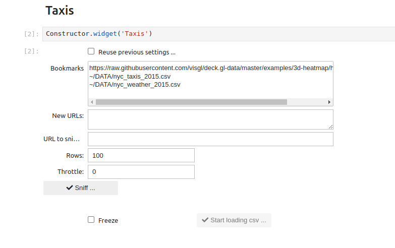
Where:
The
Bookmarksfield displays the contents (previously filled in by hand) of thebookmarksfile in$HOME/.progressivis. Lines selected here represent URLs and local files to be loaded. You can select one or more lines in this field. You can also ignore it and use the following field:New URLs: if the URLs or local files present in bookmarks are not suitable, you can enter new paths hereURL to sniff: Unique URL or local file to be used by the sniffer to discover data. If empty, the sniffer uses the first line among those selected for loadingRows: number of rows to be taken into account by the sniffer to discover dataThrottle: force the loader to limit the number of lines loaded at each stepSniff ...button: displays the sniffer (image below):

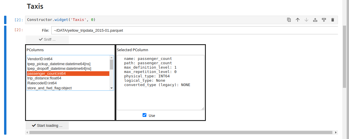
The Sniffer#
The sniffer, among other things, allows you to customize parsing options, select the desired subset of columns, and type them.
Once the configuration is complete, you can save it for later use, so you don’t have to refill all the options manually, and start loading.
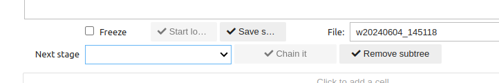
Once loading has begun, the Next stage list and the Chain it button will be used to attach a new CW to the treatments.
PARQUET Loader#
Possible topology:
Function:#
It loads one PARQUET file progressively
After starting, the main interface is:
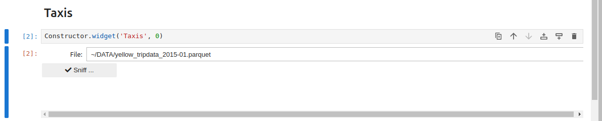
You have to activate the sniffer and select the desired columns before loading:
CUSTOM Loader#
Possible topology:
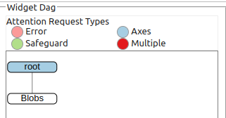
Function:#
Allows users to code their own loader in Python.
This widget is an alias for the Snippet widget, which lets you integrate portions of user-supplied code into a ProgressiBook scenario.
The only difference from the general case is that the module corresponding to the input_module parameter does not supply data, and is
useful exclusively to get the scheduler. Consequently, the widget created will always be attached to the root of the DAG.
An example is provided here. You can see that the following snippet (representing a progressive data generator) uses the input_module parameter only to obtain the scheduler:
# progressivis-snippet
from progressivis.stats.blobs_table import BlobsPTable
from progressivis.core.api import Sink

# NB: register_snippet and SnippetResult used below
# were already imported from ipyprogressivis.widgets.chaining.custom

@register_snippet
def blobs_table(input_module, input_slot, columns):
    n_samples = 100_000_000
    n_components = 2
    rtol = 0.01
    centers = [(0.1, 0.3, 0.5), (0.7, 0.5, 3.3), (-0.4, -0.3, -11.1)]
    scheduler = input_module.scheduler()
    with scheduler:
        data = BlobsPTable(columns=['_0', '_1', '_2'],  centers=centers,
                           cluster_std=0.2, rows=n_samples, scheduler=scheduler)
        sink = Sink(scheduler=scheduler)
        sink.input.inp = data.output.result
    return SnippetResult(output_module=data, output_slot="result")
Table operators category#
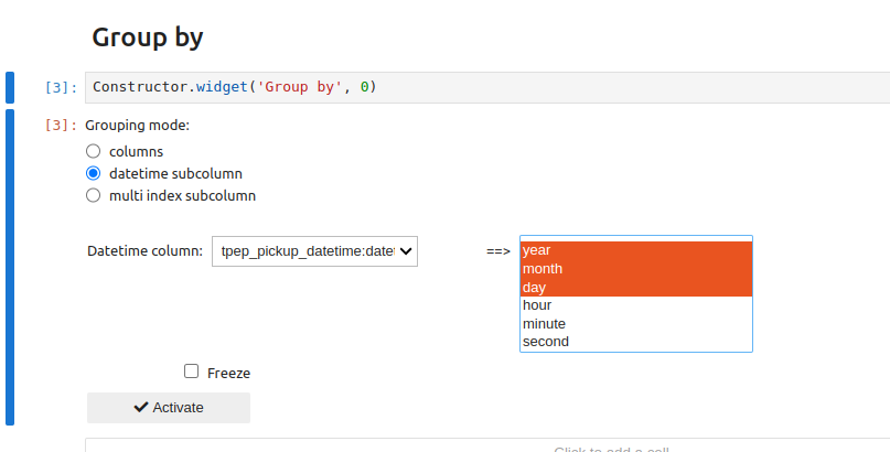
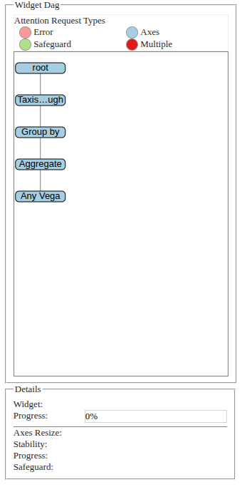
Group By#
Possible topology:
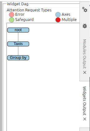
Function:#
It groups the indexes of rows containing the same value for the selected column:
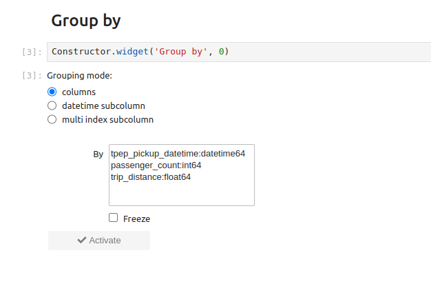
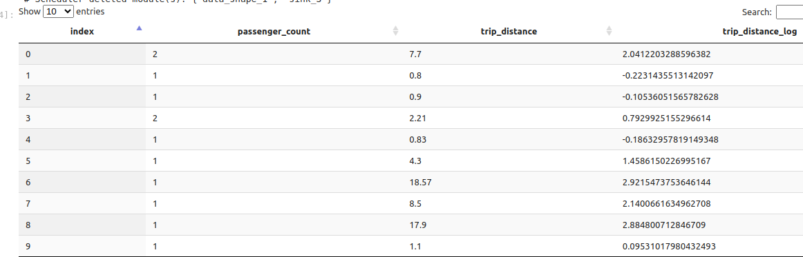
Given that tables can contain multi-dimensional values (in particular, the datetime type is represented as a vector with 6 elements: year, month, day, hour, minute, second), this CW introduces the notion of sub-columns, enabling rows to be grouped according to a subset of positions (6 sub-columns, in a datetime column). For example, indexes corresponding to the same day can be grouped together in a datetime column by selecting the first 3 sub-columns: year, month, day.
Aggregate#
Possible topology:
Function:#
Allows predefined operations to be performed on table rows previously grouped via a Group by CW:
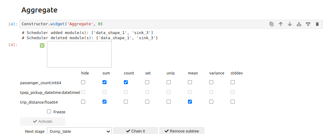
Each input (column, operation) pair generates a dedicated column in the output table:
Join#
Possible topology:
Function:#
Performs a join between two table outputs via one or more columns. Sub-column joins (in the sense described above for group-by) are also supported.
ProgressiVis currently supports one to one and one to many joins (but not many to many).
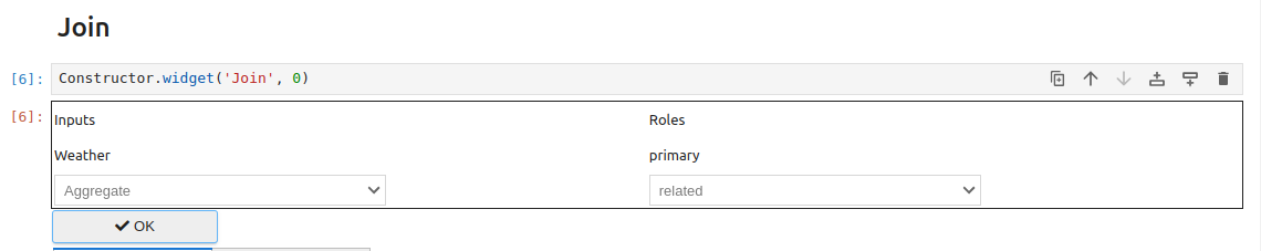
In a one-to-many join, the table on the one side is called primary and the table on the many side is called related.
Obviously, in a one-to-one join, the two roles are interchangeable:
The first step is to select the two inputs and define their respective roles, then click OK:
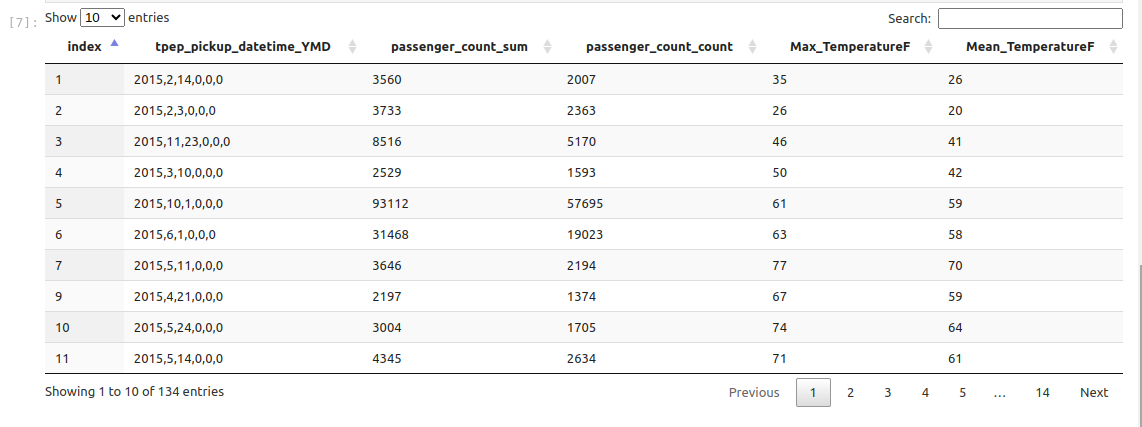
We can now define the join and select the columns to be kept in the join from among those in the primary table:
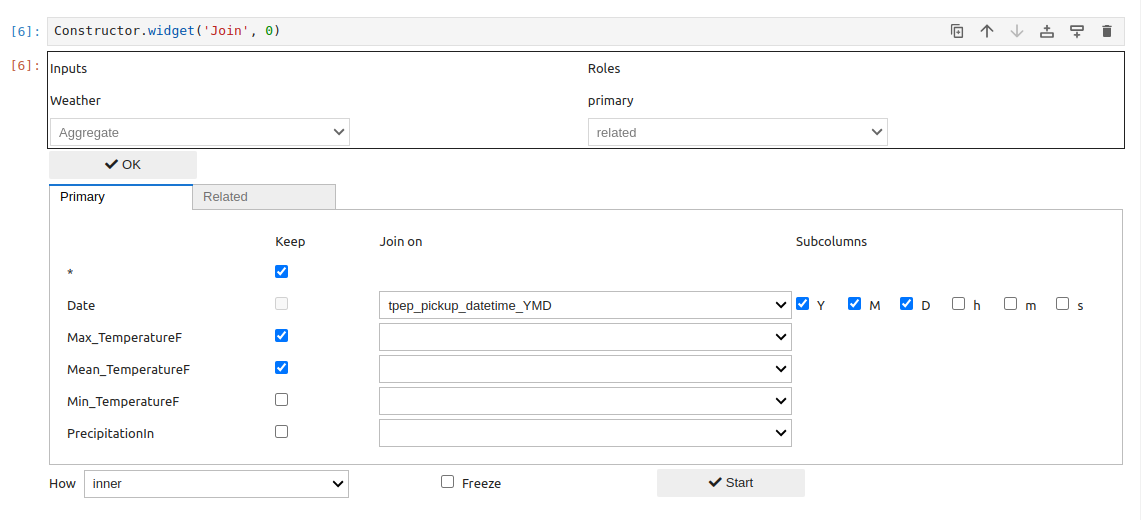
… and those in the related table:
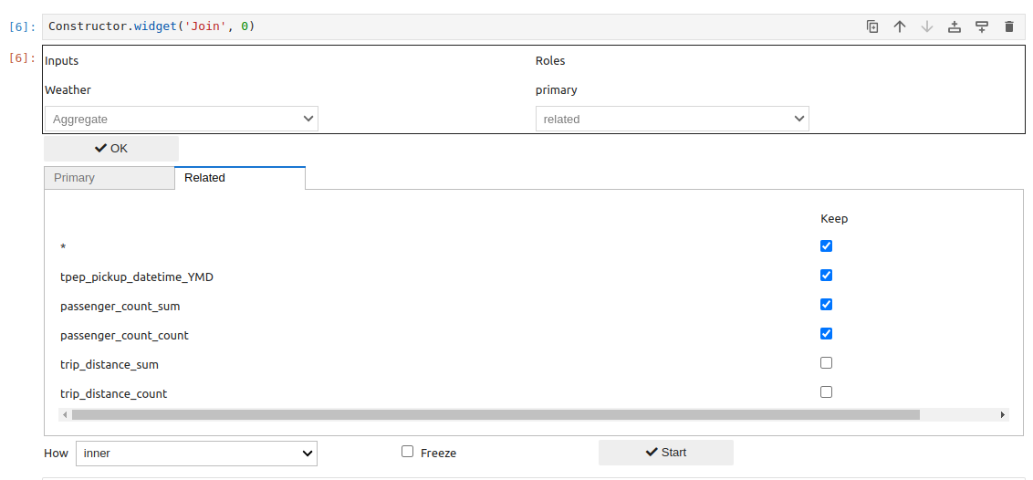
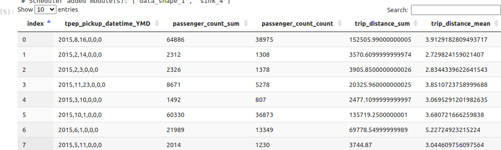
The resultant join table is:
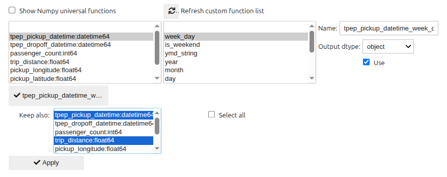
Computed View: a computed columns creator#
Possible topology:
Function:#
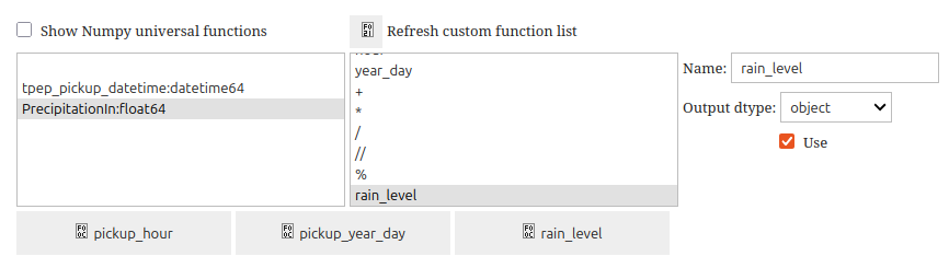
In addition to stored columns, ProgressiVis tables support virtual columns computed from the contents of other columns. Computed columns can be created programmatically or, in many cases, via the GUI shown here.
Currently these categories of functions are available:
ProgressiVispre-defined functionsuser defined
pythonfunctionsnumpy universal functions
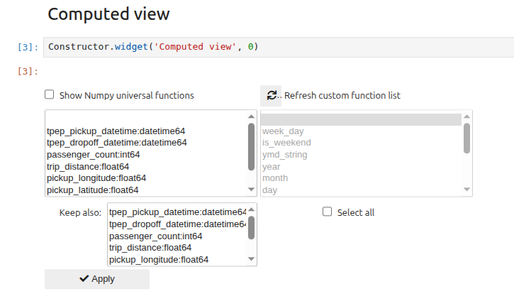
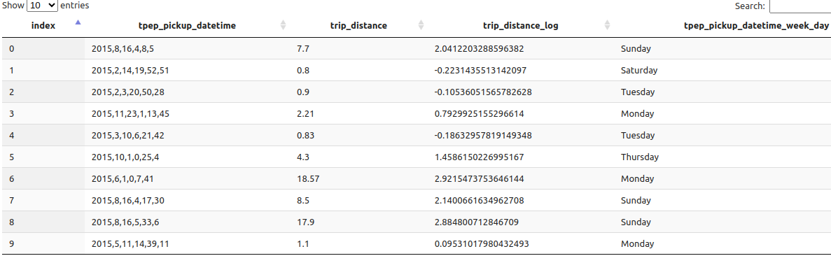
An example involving a ProgressiVis pre-defined function is the creation of a column providing the (human-friendly) weekday from a stored datetime column:
which produces the following result:
Also, user can define a function in a regular cell (see Free code section for more details):
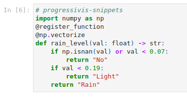
then apply it to a stored column to create a new, computed column rain_level:
As numpy functions are numerous, they are not active by default in order to lighten the presentation. In this way, only ProgressiVis and user defined functions will be displayed.
But if you check “Show numpy universal functions” they are proposed in the function list. For example, if you want a new column representing the logarithm of another stored column, you can proceed as follows (note that other stored columns can be selected to appear as they are in the result view):

giving the following result:
Free coding category#
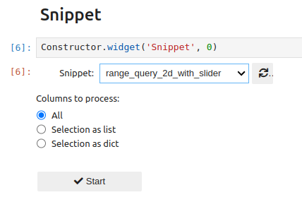
Snippet#
Possible topology:
Function:#
This is a widget that lets you insert custom code into a CW topology.
The user code must first be imported or defined in one or more cells. To be usable by the system, it must respect a few simple conventions:
the first line of each cell must begin with the comment
# progressivis-snippetThe user code must be made accessible through a function that respects the following signature:
def name_to_be changed(input_module: Module, input_slot: str, columns: list[str]) -> SnippetReturn | None:
    ... # the typing is optional but recommended
this function must be decorated with the
@register_snippetdecorator already imported into the runtime context fromipyprogressivis.widgets.chaining.custom:
@register_snippet
def my_fonction(input_module: Module, input_slot: str, columns: list[str]) -> SnippetResult | None:
    ...

# or

from my_module import my_function
register_snippet(my_function)
the function must return a
SnippetResultobject (the underlying class is already imported into the runtime context fromipyprogressivis.widgets.chaining.custom) or None if it implements a “leaf” component.
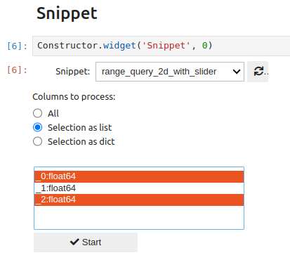
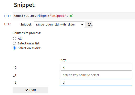
The widget lets you choose how columns will be passed to the snippet function (all, a selection of columns as a list, a selection as a dictionary):
By selecting a list, a multiple selection is proposed:
If a dictionary is chosen, keys must be entered for the selected columns:
Two complete examples are provided here. The first one is a loader (there is no input data) and the second implements an interactive range query 2D widget featuring several progressive artifacts.
CUSTOM Loader#
This is an alias of the Snippet, useful when code is not chained from another CW. This is the case for custom data loaders explained here
Other custom functions#
Some widgets can use user-defined functions (e.g., View, GroupBy, and Aggregate).
To be visible in the interface of the underlying widgets, these functions must respect a few conventions:
like snippets, they must be defined or imported in cells beginning with the comment
# progressivis-snippetthey must be decorated with the
@register_functiondecoratortheir signature must comply with the requirements of the addressed ProgressiVis module.
A complete example is provided here.
In the underlying function definition:
# progressivis-snippets
import numpy as np
@register_function
@np.vectorize
def rain_level(val: float) -> str:
    if np.isnan(val) or val < 0.07:
        return "No"
    if val < 0.19:
        return "Light"
    return "Rain"
We can see that the rain_level function is decorated with @register_function to be visible for widgets. On the other hand, its vectorization (via @numpy.vectorize) is a requirement of the underlying progressivis feature.
Display tools category#
Dump table#
Possible topology:
Function:#
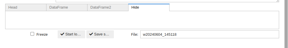
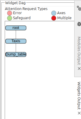
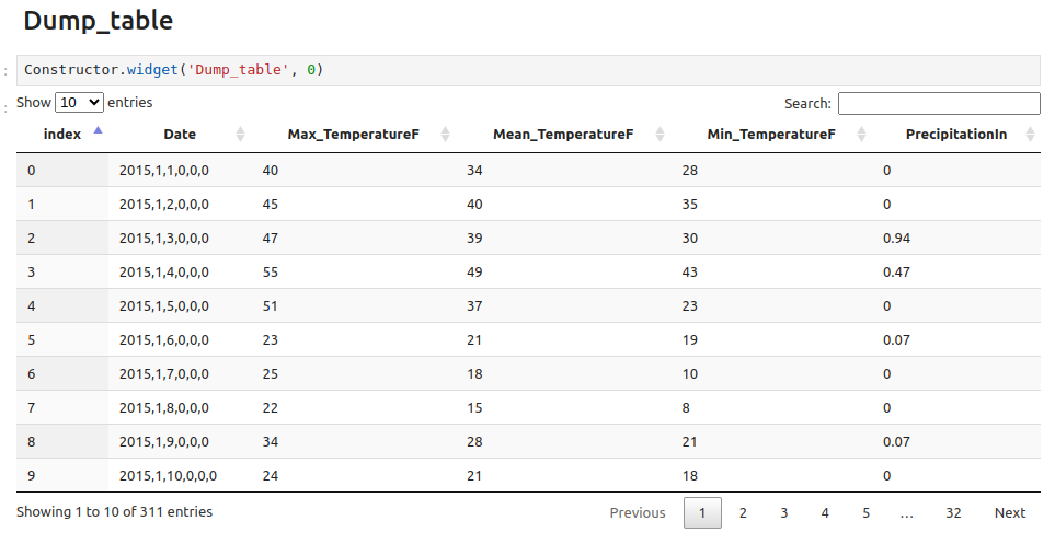
This is the simplest chaining widget that requires no configuration. It is used to display progressive table outputs and has already been used to illustrate the outputs of the widgets presented above.
Any Vega#
Possible topology:
Function:#
Allows a user to integrate Vega-based visualizations from customized schemas into a scenario. Schemas can be edited, saved, and reused in a similar way to CSV loader settings.
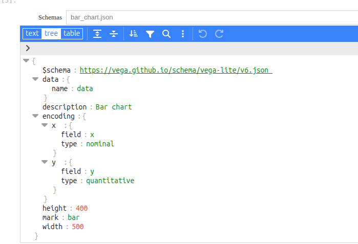
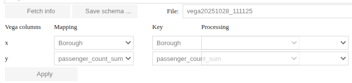
The “fetch info” button extracts the list of fields present in the schema before pairing them with members of the input module and associating them (potentially) with element-wise processing operations.
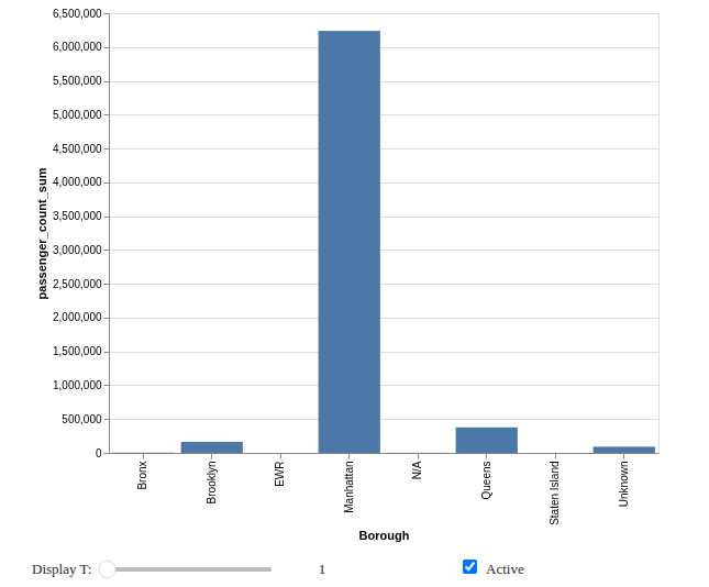
The rendering is similar to previous ones:
Recording a scenario#
A ProgressiBook lets you save a scenario for later replay. The record is persistent and it is contained in the ProgressiBook itself, so it’s a good idea to save it at the end of the recording (even if Jupyter does automatic backups periodically).
The scenario is saved only if the corresponding checkbox (named “Save this scenario”) in the start widget is checked, and it is done by default. The choice must be made before starting.
After that, the scenario is built as explained above.
NB: Scenario registration should not be confused with the persistent settings of certain widgets, which are saved in dedicated files and can also be used in unregistered scenarios.
Note
Scenario registration should not be confused with the persistent settings of certain widgets, which are saved in dedicated files and can also be used in unregistered scenarios.
Replay a scenario#
After opening a ProgressiBook containing a backup and clicking the Run ProgressiVis button, the dialog box below appears:
Once a scenario has been recorded, there are two ways to reuse it:
read-only mode
read/write mode
Both read-only and read/write modes support two alternatives:
replay all
step-by-step
In the replay all variant, all nodes in the backup are executed without any further interaction with the user (apart from those required by the scenario widgets themselves).
In the step-by-step variant, a dialog is initiated with the user, and the nodes are activated one after the other when the operator presses the corresponding Next button.
Replay in read-only mode#
This is the default mode. To keep it, leave the Allow overwriting record box unchecked. In this mode, the scenario will be replayed identically, and the backup remains unchanged. When the scenario is replayed step-by-step
Only the Next button is active since the Edit and Delete buttons are grayed out.
When replay all is chosen, chaining bars are absent on nodes, so no modification of the graph is possible.
In this mode, widgets are replaced by snapshots taken at the moment of widget creation, and they may not reflect the exact state of the configuration. Step-by-step is mainly useful for observing and understanding graph generation in a decomposed way.
Replay in read/write mode#
This mode is active when the Allow overwriting record box is checked.
In this mode, the replay all variant takes place in much the same way as in the previous mode, but each node has a bar that allows you to enrich the scenario with new nodes, as you did in the creation stage.
The step-by-step variant lets you intervene on existing nodes to modify certain parameters:
By clicking the
Editbutton, the configuration widget associated with this node will appear, allowing complete reconfiguration of the node. The user must ensure that the new configuration is consistent with further processing because the action is irreversible.By clicking on
Delete, the node in question and all its descendants will be deleted. Once again, the user must be certain of the validity of the operation, as it is irreversible.If the current node is to remain unchanged, click
Nextto continue.
Chaining widgets’ persistent settings#
CWs keeps track of its states and history with a file tree located in the user’s home directory with the following structure:
.progressivis/
├── bookmarks
└── widget_settings
    └── CsvLoaderW
        ├── taxis
        └── weather
    └── ParquetLoaderW
        ├── iris
        └── penguins
    ...
    ...
NB: Only the .progressivis directory needs to be created by the user. All other directories and files will be created by widgets as required.
How to create a chaining widget?#
Coming soon …